Finding the Non-Linear Feature: BlueDot’s Technical AI Safety Puzzle
BlueDot Impact recently ran a technical AI safety puzzle alongside their course. The setup: a small neural network trained to predict eight binary features simultaneously from short text inputs — things like “contains a person’s name”, “mentions a food”, “phrased as a question”. After a particular hidden layer, seven of those features are represented linearly in the activation space. One is not. The puzzle asks you to find it, explain the geometry, and then train a model with an even weirder representation.
I had a good time with this. A lot of the conceptual background was familiar from the Technical AI Safety course, but the hands-on analysis pushed me into techniques I hadn’t tried before. The code for the ring model and geometry analysis is on GitHub.
Finding it with linear probes
The most direct way to find a non-linear feature is to ask: for which feature does a linear classifier on the activations perform worst compared to the full model? I trained a logistic regression on the layer-2 activations (the 64-dimensional post-ReLU output of the second hidden layer) and measured the gap.
| Feature | Linear probe | Full model | Gap |
|---|---|---|---|
| number | 97.5% | 97.6% | +0.1% |
| question | 100.0% | 100.0% | +0.0% |
| color | 97.1% | 97.3% | +0.1% |
| food | 98.5% | 98.6% | +0.1% |
| sentiment | 98.2% | 98.2% | +0.0% |
| country | 42.9% | 96.4% | +53.5% |
| person | 99.8% | 99.9% | +0.1% |
| body_part | 98.0% | 97.9% | −0.1% |
Country is the obvious outlier. Seven features sit within 0.1% of the full model; country has a 53.5-point gap. The full model can detect it at 96.4% accuracy, but a linear classifier on the same activations barely beats random. Something non-linear is going on.
Finding the geometry
Knowing which feature was non-linear was the easy part. Understanding how it was represented took longer.
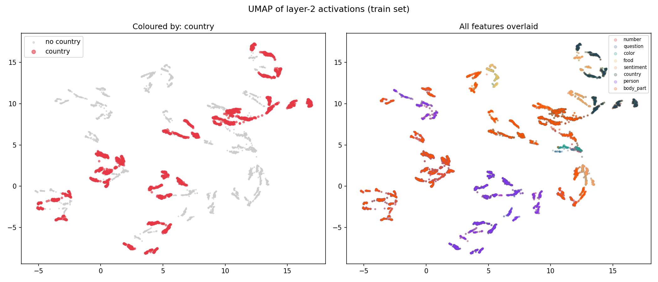
I started with visualizations — UMAP, pairwise dimension plots — hoping a picture would jump out. Some had hints of structure, but nothing obvious enough to build an explanation around.
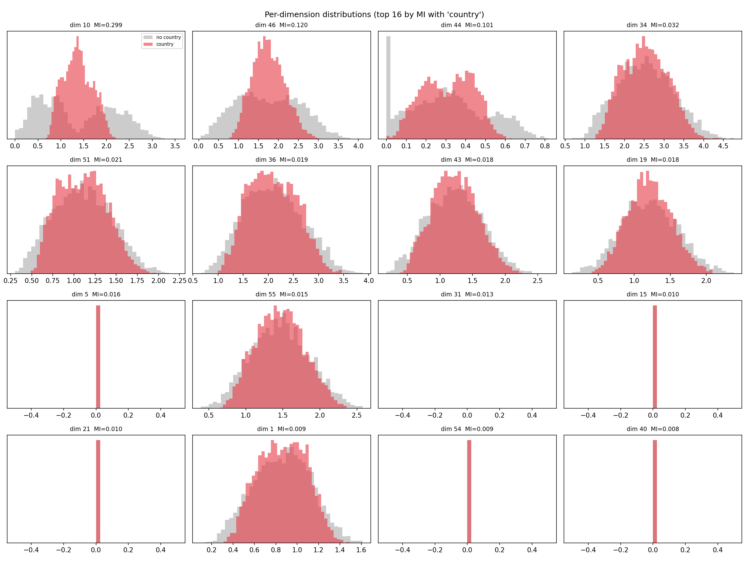
I moved on to dimension histograms and mutual information heatmaps, which showed that a handful of dimensions had elevated MI with country (dim 10 most notably, at MI=0.299), but that alone didn’t explain the geometry.
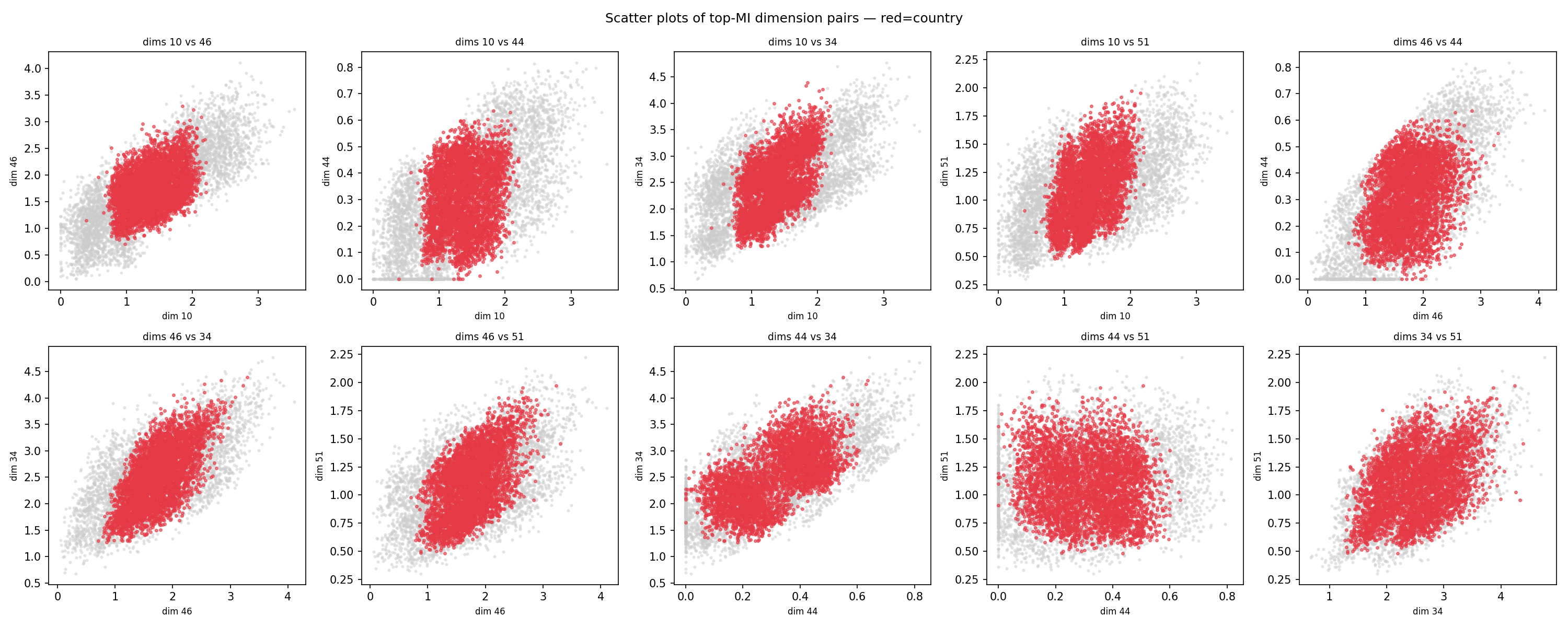
The breakthrough came from looking at superposition. I colored every example by its joint label across two features — neither / A-only / B-only / both — and plotted pairs of dimensions. For most feature pairs the four groups were scrambled. For food × country, a clear four-level ordering appeared across several key dimension pairs (10 vs 44, 10 vs 46, etc.). The examples weren’t clustering by country alone — they were clustering by the food × country combination.
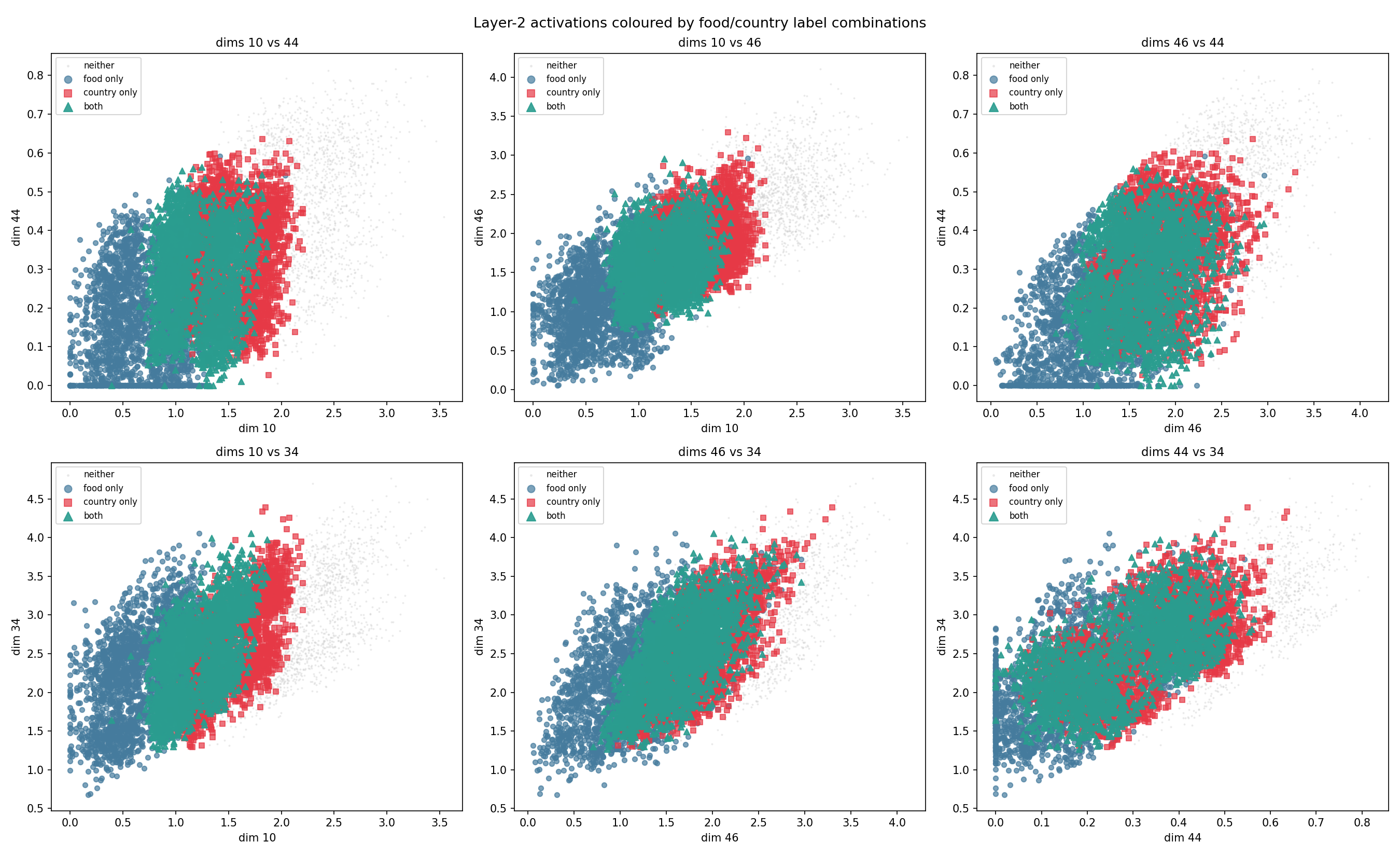
That suggested country and food were sharing a single activation direction. I projected all 8,500 examples onto the shared LDA direction and plotted density histograms for the four groups:
| Group | Median projection |
|---|---|
| neither | 0.0104 |
| country only | 0.0148 |
| both | 0.0173 |
| food only | 0.0214 |
The ordering is unambiguous, and the structure is clear: 100% of country-positive examples fall strictly between the medians of neither and food-only. Country occupies the middle interval of the shared axis — bounded above by food-only and below by neither.
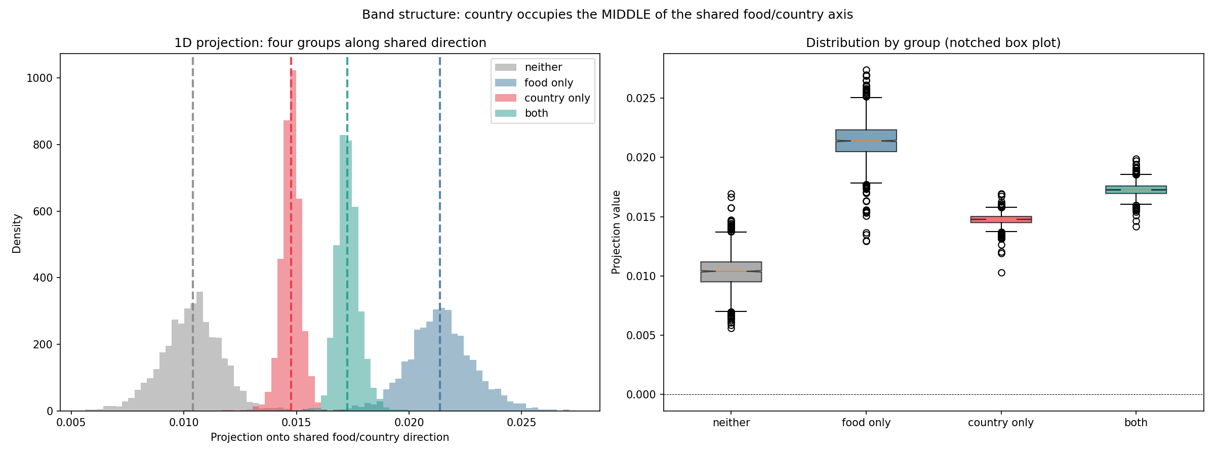
This is why a linear classifier fails. To read off country from this axis, you’d need to fire only when the activation is in a specific middle band — not above a threshold, not below one, but between two of them. That’s a bandpass filter, and it’s inherently non-linear. The network implements it using ReLU-gated suppressor units in the subsequent layers.
A weirder representation: 2D ring encoding
For part three — train a model with an even weirder internal representation — I wanted to produce something visually striking. Having spent a lot of time staring at activation space hoping a picture would emerge, I decided to try to build one on purpose.
I went with a donut. The feature is defined geometrically: given 2D coordinates (h₁, h₂) drawn from a Gaussian, the label is 1 when the radius falls in a specific annular band (0.7 < r < 1.7). This is non-linear by construction — no linear classifier can separate a ring from its interior and exterior.
I embedded these 2D coordinates into 64 dimensions via a random linear map with noise, to match the puzzle’s layer-L dimension, then trained an MLP with a 2-neuron linear bottleneck — a layer that forces all information through a 2D representation before expanding back out:
encoder
  Input(64)
  Linear → ReLU
  Linear → ReLU
  Linear(64, 2)   [bottleneck]

decoder
  Linear(2, 64)
  Linear → ReLU
  Linear → ReLU
  Linear(64, 1)
| Accuracy | |
|---|---|
| Full model | 93.9% |
| Majority-class baseline | 56.2% |
| Linear probe on bottleneck | 62.3% |
| Linear probe on true (h₁, h₂) | 56.2% ≈ baseline |
| RBF SVM on bottleneck | 93.8% |
| MLP on bottleneck | 93.6% |
The linear probe on the true coordinates sits at baseline — confirming the ring is geometrically non-linear regardless of representation. The full model and all non-linear probes reach ~94%.
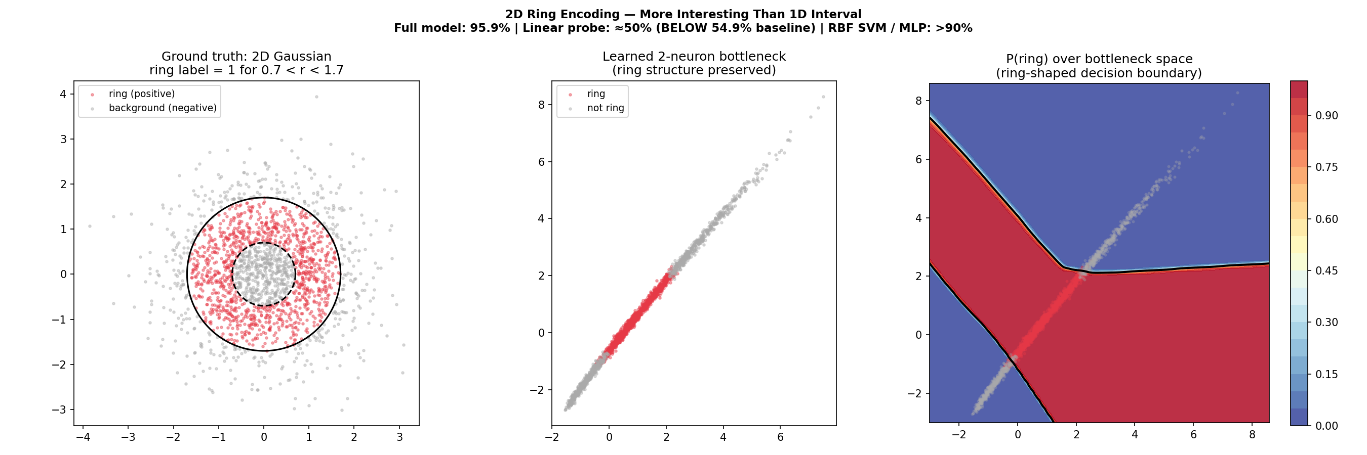
The interesting result is what the model learned to do with the bottleneck. The ring examples end up occupying a distinct band in the 2D bottleneck space — neither at the low end nor the high end, but between the two populations of non-ring examples (inside the annulus and outside it). The decoder then learned a curved decision boundary around that band, with high P(ring) in the central region and near-zero probability on either side.
This is the same band structure as the country feature, just engineered on purpose instead of discovered. The 62.3% linear probe accuracy (well above the 56.2% baseline) reflects the same phenomenon: a linear classifier can put a threshold somewhere useful, but it can’t implement a bandpass. The full model’s decoder can.
None of this was explicitly regularized. The 2-neuron bottleneck made it the path of least resistance: with only 2 dimensions to pass information through, the model settled on a representation where the ring examples cluster together, and the decoder learned to read off that structure non-linearly.
What I took away
The country feature result is a nice concrete example of superposition — two features sharing a direction — combined with non-linear readout. Seven features get their own clean linear directions; country and food share one, with country carved out of the middle. The model can decode this perfectly well using non-linear layers, but it’s invisible to any linear analysis of that layer’s activations.
The ring model is a toy illustration of something broader: you can engineer a neural network to represent a feature in an arbitrarily complex geometric structure, and as long as the subsequent layers are expressive enough, the model can learn to decode it. The bottleneck just makes the geometry visible.
I’ll admit I leaned pretty heavily on Claude Code for the ring model implementation. This was also my first time doing this kind of activation-space analysis from scratch, and I’m sure there are cleaner ways to approach some of it. But it was a fun puzzle, and I got to experiment with several techniques I hadn’t tried before. The reconstructed code is on GitHub if you want to run it.